The Model

As already described in the introductory chapter, there are numerous mangrove forests in the Exmouth Gulf. With the help of MANGA, the growth dynamics of the mangroves are reproduced in a model. The main focus is on the structure typical for mangrove forests and the dominance of individual mangrove species under different site conditions. In addition to the growth behavior of the mangroves, the salinity of the porewater - also as a sensitive parameter influencing growth - is considered in more detail. In this context the interacting influences of mangrove growth and gradients of salinity in porewater are also considered. This chapter describes the composition of the model, the basics of modeling with MANGA, and the results of the study.

Model Domain

A 185 m long and 10 m wide transect is represented in the model (Figure 1). Allometry data from a transect measurements, as well as measurement results from a long-term study, are used to evaluate the model results. The long-term study documents the effects of fertilization on the growth of 72 mangroves, half of them are located on the landward and half of them on the seaward side of the transect (see also Figure 4).

The model shows the mangrove growth at the location in the Exmouth Gulf shown in the following figure.

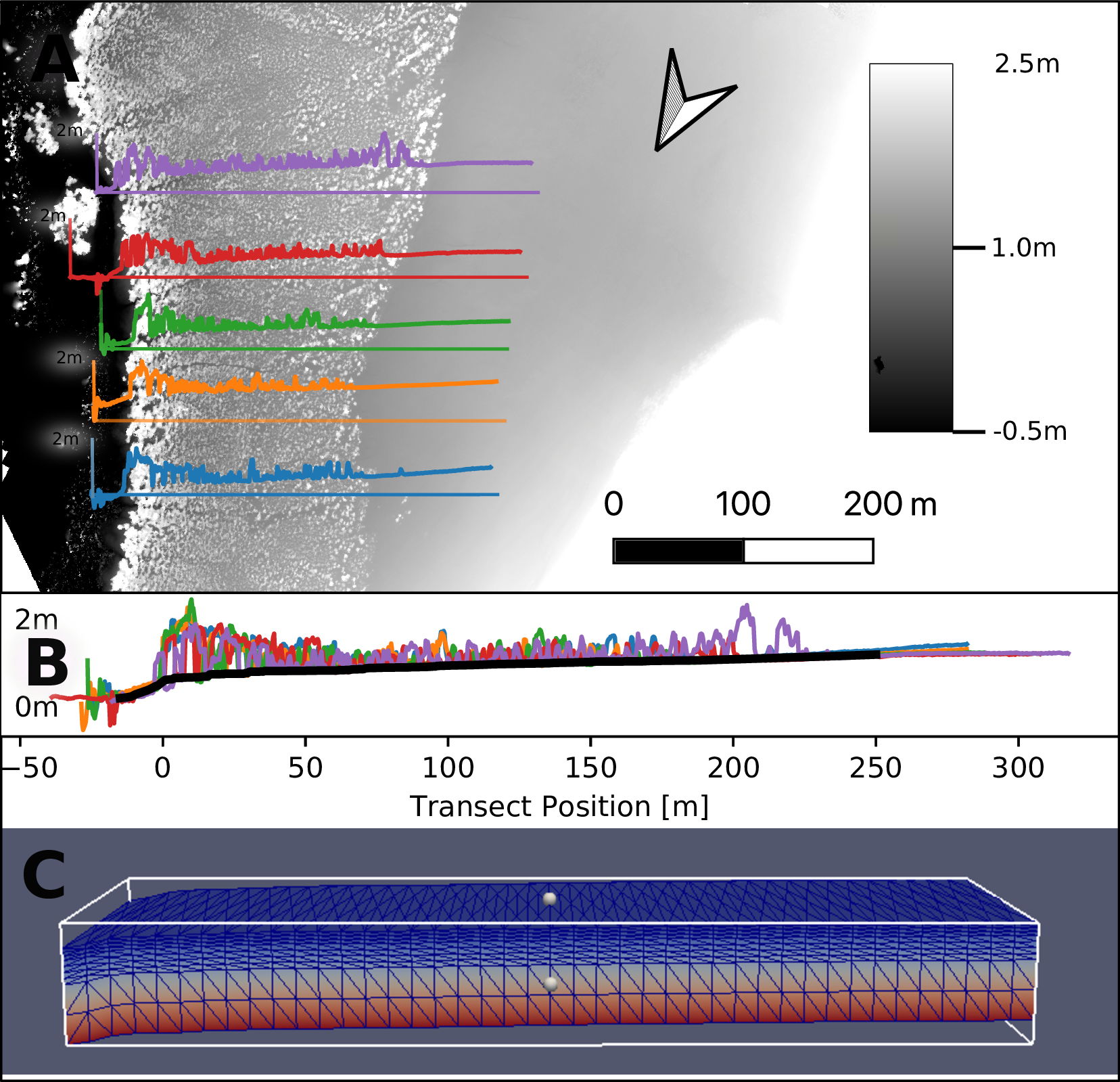
Elevation profiles from the digital elevation model of the five transects (Figure 2 A) were overlaid and the top of the terrain from the five signals (Figure 2 B) was interpolated from the baseline of the signals. This DEM was used for descretization of the groundwater model (Figure 2 C).

Modeling

Model variants

Mangrove growth was simulated using three different models (see also Table 1).

In the model “Model Without Feedback” the dynamic changes in abiotic influences (tides, groundwater recharge and salinity of seawater) are included via boundary conditions. The influence of plant water extraction on porewater salinity was not accounted for.

The model “Model Without Tide” considers the effects of plant water extraction on the salinity of the porewater and all abiotic influences of the first model - with exception of the tides.

Finally, the third model variant “Full Model” reproduces both, the dynamics of tides and the coupling of plant water extraction and porewater.

The following Table 1 summarizes the specifications of the three model variants.

	Tides	Coupling plant water balance and porewater	Other abiotic factors
Model Without Feedback	✔	✘	✔
Model Without Tide	✘	✔	✔
Full Model	✔	✔	✔

Discretization

Groundwater model

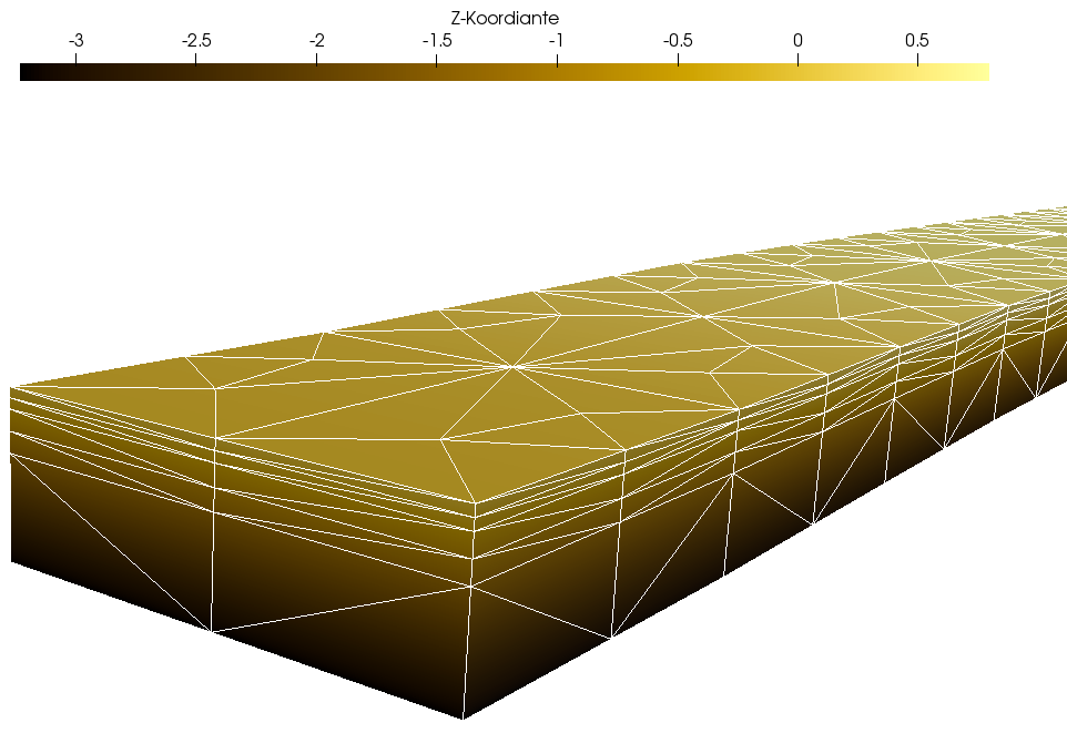
The groundwater model represents the subsurface with a grid of dimensions of 10 m x 230 m x 3 m on five FEM layers with 5880 cells. The following Figure 3 shows the spatial discretization from the seaward perspective.

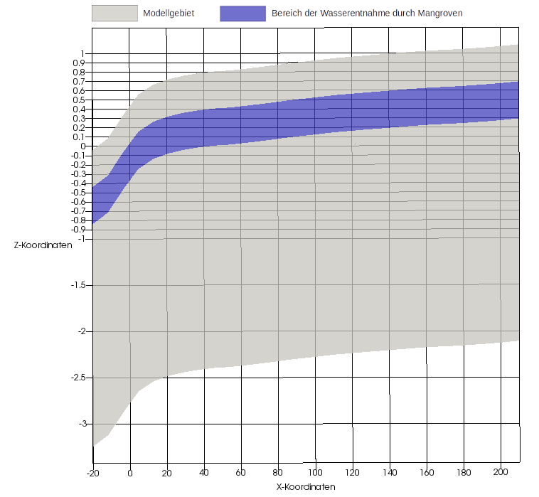
The mangroves extract soil water from the subsurface from a depth of 40 cm to 80 cm below the ground surface. Figure 4 shows the model area (gray) and the area of water extraction by the mangroves (blue). Note the 50-fold vertical scaling.

The groundwater model is discretized in time with a step length of one hour. The tidal range as a dynamic boundary condition is represented with the time series of the years 1991 to 1993, which is set in loops over the entire model runtime.

Tree growth model

Since each mangrove is represented as a single individual, there is no real spatial discretization. Temporally, the tree growth model is discretized with a time step length of half a year (1 a = 365.25 d).

Boundary conditions groundwater model

The salinity of the seawater was set at 50 g/kg, the pore water at the landward end of the transect was assigned a salinity of 70 g/kg. The transpiration of the mangroves locally increases the salinity. The water level is determined in terms of hydrostatic pressure at the seaward and landward ends of the model area. In order to represent the tides, the lake-side water level was integrated into the model as a dynamic Dirichlet boundary condition. The water level measurements of the Department of Transport of the Government of Western Australia served as data basis. The land-based water level is represented by a constant Dirichlet boundary condition. Evaporation of the trees is integrated by sink terms in the area of the roots (see also Figure 4). Inflow in the form of precipitation is indirectly considered via salinity at the landward edge of the model area. The model boundaries which are not mentioned explicitly, are all defined as no flow boundary conditions. Figure 1 shows a schematic diagram of this.

Parameterization

The following tables show the parameterizations of the subsurface (Table 2) and the mangroves (Table 3), global weighting factors (Table 4), and the initial values of the geoemtries of the mangrove seedlings (Table 5).

Subsurface

Table 2: Parameterizations of subsurface

Symbol	Parameter Name	Value
Dm	Molecular diffusion coefficient	1 × 10-9 m2/s
βT	Transversal dispersivity	0.5 m
βL	Longitudinal dispersivity	1 m
ρ	Water density	1 × 103 kg/m3
μ	Dynamic Viscosity	1 × 10-3 Pas
κ	Intrinsic permeability	5 × 10-11 m2
Φ	Soil porosity	0.5

Botany

Water balance of the mangroves

Table 3: Parameterization of the biotic factors

Symbol	Species parameter	Avicennia marina	Rhizophora mangle
Dm	Leaf water potential	-8.15 × 106 kg/s2/m	-6.45 × 106 kg/s2/m
kf	Xylem conductivity	1.04 × 10-10 kg/s/m2	3.12 × 10-10 kg/s/m2
Lp ⋅ kgeo	Fine root permeability ⋅  scaling factor	1.32 × 10-11 kg/s/m4	1.32 × 10-11 kg/s/m4
km	Maintenance cost per biomass	1.4 × 10-6 kg/s/m3	1.4 × 10-6 kg/s/m3
kgrowth	Growth speed scaling	3.5 × 10-3	3.5 × 10-3

Global weighting factors

Table 4: Global weighting factor

Symbol	Global weighting factor	Avicennia marina	Rhizophora mangle
CS	Solar resource inputs	5 × 10-8 kg/s/m2	5 × 10-8 kg/s/m2
σ	First sigmoidal slope	1.5 × 10-2	1.5 × 10-2
σh	Second sigmoidal slope	5 × 10-2	5 × 10-2
ωh	Heigth growth scaling factor	0.12	0.12

Initial values of the geometrical characteristics of the mangrove seedlings

Table 5: Initial value of the geometrical characteristics of the mangrove seedlings

Symbol	Geometric measure	Avicennia marina	Rhizophora mangle
rR	Root radius	0.25 m	0.25 m
rC	Crown radius	0.3 m	0.3 m
rS	Stem radius	0.01 m	0.01 m
hR	Root depth	0.015 m	0.015 m

Resource competition

For representing the mangroves in the model area, it is necessary to establish a stable population, which means to reach quasi-stationary conditions. For this purpose, 30 mangroves are randomly positioned in the model area as seedlings. In each time step (length: half a year), 30 new mangroves are added, which are also randomly positioned in the model area. Due to the competition-based tree growth model, these new mangroves die more or less quickly. Thus, the probability that a young mangrove in the catchment area of an already older one dies again very quickly is very high. The reason for this is the above-ground competition, especially the lack of sunlight. Due to the concentration of salinity, caused by extraction of fresh water from the other mangroves, salt plumes are formed in the pore water. These lead to growth penalties for the mangroves located downstream (especially for young mangroves). Different mangrove species have varying tolerance to high salt concentrations. In this research, the two species Avicennia marina (“gray mangrove”) and Rhizophora mangle (“red mangrove”) were studied in more detail.

Results

In this research, two processes were viewed more closely with the help of the MANGA model. On the one hand, the development of typical structures in mangrove forests is be mapped, on the other hand, the growth behavior of the two mangrove species under different environmental conditions is investigated. In the following the results of the research are briefly summarized.

Forest structure

The following visualization shows the dynamic development of the mangrove population in the model area and the development of the biomass. The increasingly stable mangrove population can be clearly seen in the first 100 time steps. Over the X-length of the transect are relatively quickly building areas in which large and thus very old mangroves grow, and areas in which young mangroves quickly die again. Due to the fact that 30 new mangroves are added to the model as seedlings in each time step and the nutrient competition is initially very low, the biomass in the model initially grows very strongly. As the number of mangroves in the model area increases, the competition between individual trees increases, too. After the global maximum of the biomass, the biomass decreases slightly due to worsening nutrient conditions for some mangroves. After a certain time, a quasi-stationary state of the mangrove population is reached.

  Timestep:      

0

  

In the following video the model area was divided into ten sectors. The dynamic development of the mangrove population and the salt concentration in the bottom water as well as the biomass of the mangroves in the individual sectors are shown. Compared to the previous visualization, one main cause of the formation of the typical forest structure can be seen in this video, namely the concentration of salinity in the pore water in certain areas. The high correlation between salt concentration and biomass in the individual sectors can be seen already from a model runtime of 40 years. Already from 100 years, the structure of typical mangrove forests is recognizable.

The results of the “Full Model” are in qualitative agreement with the measured field data (Figure 5). This is true for both the tree height profile (Figure 5 A) and for the porewater salinity profile (Figure 5 B) in the studied transect. In particular, the variation in porewater salinity was well mapped (Figure 5 A). The coefficient of determination of the Bravais-Pearson correlation is R² = 0.64 for tree height and R² = 0.88 for porewater salinity. A comparison of the results of the “Full Model” with the results of the two model variants “Model Without Feedback” and “Model Without Tide” shows a significantly worse reproduction of the measured field data by the two simpler models (Figure 5 C and 5 D).

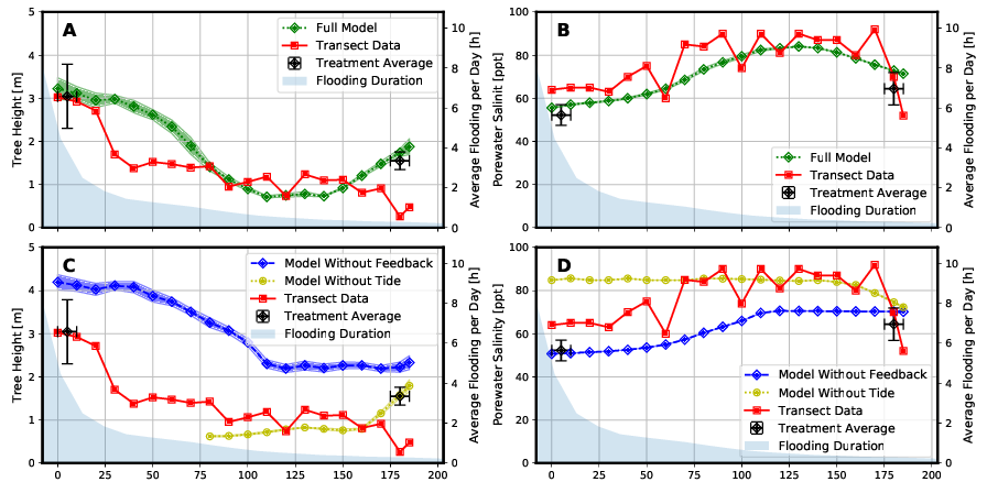
The “Treatment Averages” plotted in Figure 5 are from mangroves that have been studied in more detail in long-term experiments. A comparison of the results of these observations with the modeling results also shows a high degree of agreement.

In order to investigate the effects of the temporal dynamics of tides and plant water extraction on the salinity in the pore water, this effect was normalized using the following formula:

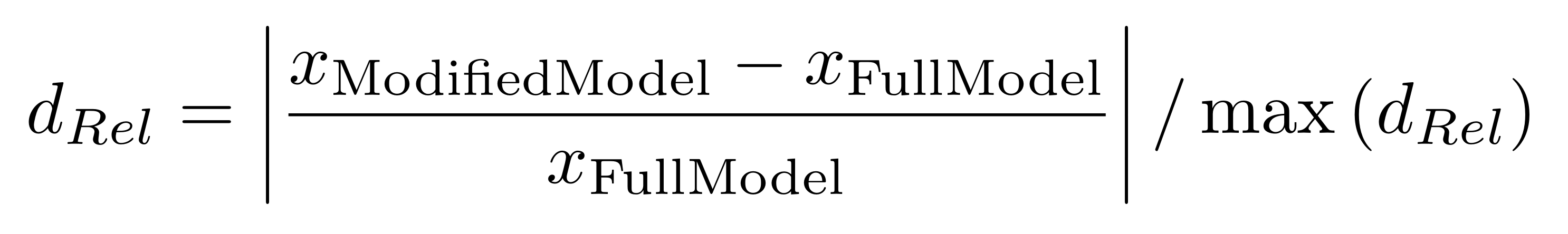
These relative effects are shown in the following Figure 6 for tree height and porewater salinity. A value of zero would mean that there is no difference in results between Full Model and the respective simplified model type. The larger the value becomes, the higher the deviation.

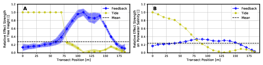
Due to the greater effects of the tidal range in the area close to the sea, the model “Without Tide” can only represent the tree heights and the porewater salinity here with a relatively large deviation compared to the “Full Model”. However, with further inlands, the water level fluctuations due to tides become smaller. Tree heights and salinities can be represented in this range (x > 75 m) with smaller relative deviations from the “Full Model”.

The Model “Without Feedback” fails to predict mangrove growth height as the “Full Model” does, especially in the middle to landward area (60 m < x < 165 m) of the transect. In this area the salinity of the porewater is concentrated by the plant water extraction, but this is not represented in this type of model.

Species dominance

In the previous section, it was shown that MANGA, with the consideration of salinity in the bottom water and the tidal range, is able to represent the forest structures typical for mangrove forests. Using the extensive parameterization capabilities of the tree growth model (see also the section parametrization), MANGA can also be used to study the growth of single specific individual species. For example, different mangrove species have different tolerances to excessive salinity. In this project, the growth behavior of two species, Avicennia marina and Rhizophora mangle, was studied in more detail.

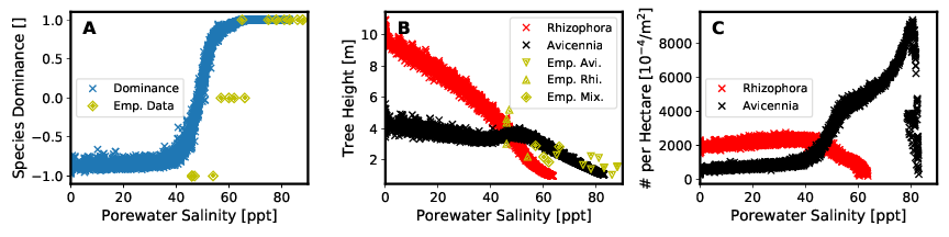
Figure 7 shows the species dominance of these two mangrove species at different salinity concentrations (see Table 6) in porewater. The different setups shown in the figure differ only with respect to the boundary conditions of the seaward and landward salinity concentrations of the porewater. For the consideration of species dominance in the model domain, we introduce the species dominance d and define it as follows:

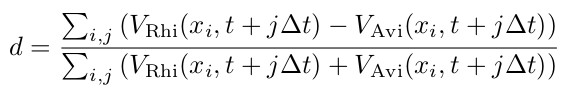
Here, V_i(x,t) represent the volume of mangrove species Rhizophora mangle (V_Rhi(x,t)) and Avicennia marina (V_Avi(x,t)) present at the time step (t) and X coordinate (x).

Table 6: Setup configuration

Setup	A	B	C	D	E	F
seeward salinity [g/kg]	15	15	25	50	50	35
landward salinity [g/kg]	25	40	55	60	45	35

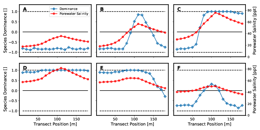
Figure 7A to 7D show an initially monospecific Rhizophora forest (Figure 7A) due to both seaward and landward low salinity concentrations. As salinity increases, a mixed forest of both species is established (Figure 7B and 7C). Figure 6D then depicts a monospecific Avicennia marina forest due to the high salt concentrations. Both Figure 7E and 7F are similar to setup configurations Figure 7B and 7C in that the values of salinities on landward and seaward sides of the transect, respectively, assume approximately the other value. Thus, they too represent a mixed forest of both species. These results are shown again in a different way in the following Figure 8.

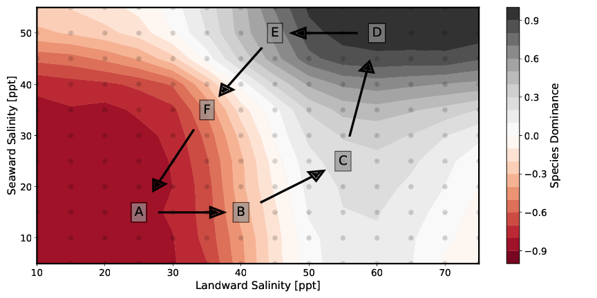
When looking at the mixed forests, real mixed populations are existing only in a few individual sections. In most areas a clear dominance of one species is expressed. These sharp transitions between the individual dominance zones show that coexistence between the different species is only possible in areas of certain pore water salinities. The location of the boundaries and the change in species dominance d (slope of the curve) depend on the individual-specific parameters in the tree growth model. Soil water salinity is also affected by the number of individuals per area and tree heights. These two parameters are in turn influenced by the same individual-specific parameters.

Consequently, the coupling between plant water balance and porewater significantly influences the formation of forest structure. In the setups that result to the formation of a mixed forest, either two-zone (Figure 7C and 7E) or three-zone (Figure 7B and 7F) mixed forests are formed. The two zones at the seaward and landward end of the model are mainly controlled by the parameters of salinity as boundary condition. In the model center, the transpiration of the mangroves leads to a concentration of the porewater salinity. If this exceeds a certain value, the more salt-resistant species Avicennia marina dominates.

As also shown in Figure 9, the results of considering species dominance in the model are consistent with the measured field data in those transects considered in the project.

Consequently, the MANGA model software is able to represent not only the evolving structure of a mangrove forest, but also its composition of different species.

Conclusion

With “Full Model” the structure which is typical for mangrove forests can be modeled. Specifically, the forest structure of the Avicennia marina monoculture forest in the considered area in the Exmouth Gulf in Western Australia could be reproduced in a consistent manner with the available field data. Variations in tree heights and soil water salinity between model and measured values are within the range of variability in field measurements. MANGA is capable of doing this without further calibration of plant-specific parameters. The “Full Model” was able to identify areas in the model area where either tides or vegetation significantly influence structural properties.

Based on the results of the modeling, it must be assumed that a correct representation of mangrove growth with MANGA is only possible if the tidal range and the influences of water extraction of the mangroves from the subsurface are considered. Calibration of the plant parameters is not necessary for this purpose. Also not considered are heterogeneous hydrogeological properties of the subsurface, e.g. concerning hydraulic conductivity or porosity.

The gradients of the salt concentration in the porewater caused by the plant water extraction have a significant effect on the growth dynamics of the mangrove population, especially in the landward area. Further, it can be concluded from the results that the influence of tides is a major influencing factor on the gradients of salinity concentration in bottom water. This influence is greatest at the seaward end of the transect. As the height of the tide decreases, or the duration of inundation decreases, the feedback between plant water and bottom water budgets takes on increasing importance in this process.

Using the sensitivity analysis of the model with respect to species dominance, it was shown that species composition can be described by considering soil water balance and plant water withdrawal across the system boundary. By variation of just two parameters (see Table 3) that directly affect tree water uptake, typical zonation patterns in mixed mangrove forests could be reproduced. This was accomplished even with roughly estimated plant-specific parameters for one of the two species. If the boundary conditions of the salt concentrations on the land- and seaward side are both chosen very high or very low, monoculture forests are formed. If a moderate mean value of the salinities is chosen, mixed forests of both species are formed. These show zones with clear dominance of one species, separated by sharp transitions. These transitions are shown to depend on the porewater salinity. The species composition in the model agrees with the measured field data.

Outlook

There is evidence in the literature that mangroves adapt to their environmental conditions over time. A lower salt concentration in the bottom water provides higher xylem conductance and thus greater transpiration. At the same time, however, a low salt concentration in the subsurface also provides higher leaf water potentials that inhibit transpiration. These mutually balancing processes provide approximately constant transpiration rates at different porewater salinities. A more detailed study of these processes may help to understand the ability of mangroves to adapt their physiology to appropriate sites prevailing environmental conditions.

Precipitation was not dynamically integrated as a separate process in this project, as still described, but is represented by the land-based constant boundary condition of water level and salinity. The Exmouth Gulf is generally a region of very low annual precipitation sums. However, the variability of individual rainfall events is very high. Due to cyclones, heavy rainfall events occur regularly and account for a not insignificant portion of the total precipitation. The influence of precipitation on the mangrove population was studied indirectly by setting different values of the boundary condition of landward porewater salinity. Since this boundary condition was shown to be a very sensitive variable, it follows that precipitation also has an influence on mangrove species composition and, in general, the formation of typical mangrove forest structures. In the course of climate change, it can be assumed that heavy rainfall events or generally extreme weather situations will increase and that sea level will rise. Since the model was able to represent the populations according to reality, it could also be used to investigate the effects of climate change on the sensitive ecosystems of the mangrove forests. Further, the model can provide important clues in the study of all relationships between forest structures and plant characteristics. Models that represent the processes based on more conceptual approaches than MANGA can be calibrated and verified with MANGA.